DESeq2 or edgeR

I was asked recently on Twitter about my thoughts on DESeq2 and edgeR and which tool is better. My reply was:

@lpachter @gordatita_ @BioMickWatson @wolfgangkhuber perform similarly. I recommend people read papers and decide themselves

— Mike Love (@mikelove) September 9, 2016

But then I was asked to elaborate more so here goes:

TL/DR summary: I think DESeq2 and edgeR are both good methods for gene-level DE, as is limma-voom.

Aside: The bootstrapping idea within the sleuth method seems especially promising for transcript-level DE, but I have only kept up with the ideas and haven’t done any testing or benchmarking with sleuth yet, so I won’t include it in this post.

History: When we started working on DESeq2 in Fall 2012, one of the main differences we were focusing on was a methodological detail* of the dispersion shrinkage steps. Aside from this difference, we wanted to update DESeq to use the GLM framework and to shrink dispersion estimates toward a central value as in edgeR, as opposed to the maximum rule that was previously implemented in DESeq (which tends to overestimate dispersion).

I would say that the difference in dispersion shrinkage didn’t make a huge difference in performance compared to edgeR, as can be seen in real and simulated** data benchmarks in our DESeq2 paper published in 2014. From what I’ve seen in my own testing and numerous third-party benchmarks, the two methods typically report overlapping sets of genes, and have similar performance for gene-level DE testing.

What’s different then? The major differences between the two methods are in some of the defaults. DESeq2 by default does a couple things (which can all optionally be turned off): it finds an optimal value at which to filter low count genes, flags genes with large outlier counts or removes these outlier values when there are sufficient samples per group (n>6), excludes from the estimation of the dispersion prior and dispersion moderation those genes with very high within-group variance, and moderates log fold changes which have small statistical support (e.g. from low count genes). edgeR offers similar functionality, for example, it offers a robust dispersion estimation function, estimateGLMRobustDisp, which reduces the effect of individual outlier counts, and a robust argument to estimateDisp so that hyperparameters are not overly affected by genes with very high within-group variance. And the default steps in the edgeR User Guide for filtering low counts genes both increases power by reducing multiple testing burden and removes genes with uninformative log fold changes.

What about other methods? There are bigger performance differences between the two methods and limma-voom, and between the GLM methods in edgeR and the quasi-likelihood (QL) methods in edgeR. My observations here are that it does seem that limma-voom and the QL functions in edgeR can do a better job at always being under the nominal FDR, although they can have reduced sensitivity compared to DESeq2 and edgeR when the sample sizes are small (n=3 per group), when the fold changes are small, or when the counts are small. Methods should be less than their target FDR in expectation, but one should always consider FDR in conjunction with the number of recovered DE genes. In my testing across real and simulated** datasets, I find DESeq2 and edgeR typically hit close to the target FDR. The only time I tell people they should definitely switch methods is when they have 100’s of samples, in which case one should switch to limma-voom for large speed increases. An additional benefit of limma-voom is that sample correlations can be modeled using a function called duplicateCorrelation, for example repeated measures of individuals nested within groups.

Ok, so what are some good papers for comparing DE methods?

I think a nice comparison paper that came out earlier this year is Schurch et al (2016). The authors produced 48 RNA-seq samples from wild-type and mutant yeast (biological replicates), where the mutation is expected to produce many changes in gene expression. Of the 48 samples, 42 passed QC filters and were used to assess performance of 11 methods for gene-level DE. Sensitivity was assessed by comparing calls on small subsets of data to the calls in the larger set, similar to an analysis we did in the DESeq2 paper in 2014. Specificity was assessed by looking  at calls across splits within a condition. Null comparisons are useful for assessing specificity of DE methods, as long as the null comparisons do not include splits confounded with experimental batch, which will produce many positive calls due to no fault of the methods***.

I think the Schurch et al paper gives a very good impression of what sensitivity can be achieved at various sample sizes and the relative performance of the 11 tools evaluated. One change I would have made if I were doing the analysis is to use p-value cutoffs to assess null comparisons, because then one can see the distribution, over many random subsets, of the number of genes with p-values less than alpha. Boxplots of this distribution should be close to the critical value alpha.

Finally, one can assess the false discovery rate (1 – precision) using a similar technique to the sensitivity analysis: comparing the proportion of positive calls in the small subset which are also called in the larger subset. It’s really a self-consistency experiment, because we never have access to the “true set” of DE genes. The Schurch paper used FPR instead of FDR, but we have such an analysis in the DESeq2 paper. As the held-out subset gets larger, this should be a good approximation to the FDR supposing that methods generally agree on the held-out set.

I took the time to update our analysis of the Bottomly et al mouse RNA-seq dataset using the current versions of software in Bioconductor (version 3.3). Thanks to Harold Pimentel and Lior Pachter, who helped me in updating my code. My original 2014 analysis did not use CPM filtering for edgeR or limma-voom, which should be used for an accurate assessment. Here I use the filter rule of at least 3 samples with a CPM of 10/L, where L is the number of millions of counts in the smallest library. I also tried using a rule of at least {min group sample size} samples with CPM of 10/L, so 7 for the held-out set, but this was removing too many genes to the detriment of edgeR and limma-voom performance.

FDR and sensitivity, comparing algorithms to their own held-out calls, for the release versions of DESeq2, edgeR and limma-voom are plotted below. The figure looks roughly similar to (1 – precision) in Figure 9 of the DESeq2 paper (thresholding at 10% nominal FDR), except the CPM filtering definitely improves the performance of limma-voom. While the estimates of sensitivity look comparable here, note that for the 3 vs 3 comparison, DESeq2 and edgeR call ~700 genes compared to ~400 from edgeR-QL and limma-voom.

 

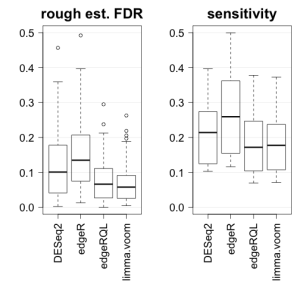
In this analysis, the larger subsets contain 7 vs 8 samples compared to the small subsets with 3 vs 3, so the rough estimate of FDR is likely an overestimate, because the 7 vs 8 comparison has not saturated the number of DE genes (see Figure 1 of Schurch et al). I would say all methods are probably on target for FDR control if the held-out set were to grow in sample size; in other words, there is still a lot of stochasticity associated with the held-out set calls. Critical to this analysis is the fact that we balance batches in all of the splits, or else the comparisons might include batch differences in addition to the difference across groups (here species).

Additionally, I looked at the overlap of pairs of methods and found that methods generally had about 60-100% overlap. When the overlap was only 60% (edgeR or DESeq2 vs limma-voom in the 3 vs 3 comparison), this typically indicated that 100% of the DEG of one method were included in the other. Meaning that one method is calling more than the other. Note that this can happen and the methods can still both be controlling FDR, because there is not a unique set of genes which satisfies E(FDR) < target. In the 3 vs 3 comparison, DESeq2 and edgeR have about 90% overlap with each other, while in the 7 vs 8 comparison, edgeR makes up about 80% of the DESeq2 calls. I looked into the extra calls from DESeq2 in the held-out set (DESeq2 called about 600 more genes than edgeR), and the majority of these were filtered due to the CPM filter, although the top genes in the set exclusive to DESeq2 were clearly DE but with low counts.

All plots for this analysis can be found here, and the code used to produce the plots can be found here.  The code for the analysis in the original DESeq2 paper can be found here.

* At that point in time (2012), the dispersion estimation steps for the GLM in edgeR used a pre-set value (prior.df) to balance the likelihood for a single gene and the shared information across all genes. We were looking to another method DSS, which based the amount of shrinkage on how tightly the individual gene dispersion estimates clustered around the trend across all genes. Two points to make: (1) the default value in edgeR performed very well and we didn’t find that our different approach to dispersion shrinkage made a huge difference in the evaluations, and (2) the recommended steps in the edgeR User Guide since 2015 anyway use a different function, estimateDisp, which estimates this value that determines how to balance the likelihood of a single gene and the information across all genes.

** A note on simulations: in my last two papers in which I was the first author, I’ve tried to avoid simulations and use only “real data” in the manuscript, but have been forced in both cases to include simulations at the insistence of reviewers or editors. I would say in both cases the simulations did prove useful to demonstrate a point (e.g. how does DESeq2 perform for a grid of sample sizes and effect sizes), but simulations should be considered only part of a story. In both cases I would have saved many months by including simulations in the first submission.

*** Wait, Mike, but didn’t you just publish a paper looking at transcript abundance differences across lab? Yes, but there is a key difference. In that work, we are trying to make abundance estimates as close to the true abundances as possible, trying to remove differences in abundance estimates across lab by learning technical features of the experiment. The ideal method would give concordant estimates across lab. Comparing estimates across lab was a way for us to identify and characterize mis-estimation.